NeRF Starter Kit: a conceptual journey

Global Models

DeepSDF and OccNet are of the pioneering works that attempted at representing 3D scenes using implicit functions with neural networks. These two papers introduce auto-decoders as an important architecture for storing a 3D scenes that is not prone to over-smoothing like auto-encoders and can store detailed scenes by not losing any information through low-dimensional encoding like AE. The NASA paper then follows the same trend for modeling articulated bodies, containing important architectural ideas on how to use and combine multiple implicit functions that model rigid bodies to arrive at a non-rigid body model.

OccNets @ CVPR 2019 – arXiv

Left: An occupancy function can be modeled as the decision boundary for classifying inside and outside points. Right: The decision boundary corresponds to a surface in 3D.

The goal here is to learn a function to map a 3D point into a continuous function which models the inside and outside of an object. OccNets trains an MLP to classify the points into inside, outside. The learnt decision boundary function can then be turned into a mesh using their introduced MISE method and a hyperparameter which thresholds the surface. MISE basically first hierarchically zooms in to the surface by gridding. Then runs a marching cube and refines it using first and second order gradients. The zoom and grid procedure helps MISE result in more detailed modeling than plain marching cubes. OccNets can be adapted into different tasks by conditioning their function on different inputs. A Resnet for image conditioning and a PointNet for pointcloud conditioning is used in the experiments. Compared to previous work which use voxel, mesh, or point cloud representation OccnNt shows much better qualitative and better quantitative results. Interestingly it is slightly over-smooth which is an inherent property of modeling with an MLP, because of the spectral bias theorem. This is reflected in inferior L1-chamfer distance compared to AtlasNet (mesh based).

DeepSDF @ CVPR 2019 – arXiv

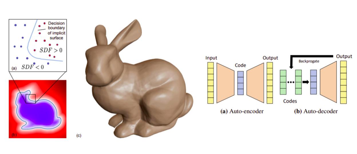Left: Signed Distance Function, Right: Auto-decoder vs. Auto-encoder

Exploring the idea of having 3D representations using neural implicit fields to achieve high quality reconstruction and compact models, this paper introduces SDF functions, a useful representation of object geometry, stored in deep networks. Given a mesh representation of an object, this method converts the mesh to a Signed Distance Function (SDF) where a point inside the object has negative value, zero on the surface and positive outside. The main idea is to use an auto-decoder (decoder + latent codes), that takes as input point coordinates and a shape latent code and outputs SDF value. The decoder weights and shape codes are optimized using MAP during training and in test time only the shape code is optimized. Directly optimizing latent codes in an auto-decoder helps capture finer details and generalize to test objects better, while in an auto-encoder setting the encoder always expects to receive inputs similar to what its seen at train time. Therefore in an auto-encoder some info and details are lost through encoding to lower dimensions while optimizing latent codes directly can overfit better to the given input.

NASA @ ECCV 2020 – arXiv

NASA: three different models of non-rigid body. The explicit conversion of coordinates is done prior to mapping to occupancy through a decoder.

Implicit neural representations for articulated and non-rigid bodies is an interesting problem that is addressed in this paper. NASA uses an occupancy net for articulated bodies and progressively presents 3 models of body, where in first one the body is a rigid object (U), then a piece-wise rigid object (R) and finally deformable (D). In R model, the query coordinates are transformed to each rigid piece’s canonical frame, while in U model the whole body is considered one rigid object and query points are canonicalized based on the main body frame. This paper shows the importance of converting coordinates to canonical frame before passing it into an MLP (in this case query/joint coordinates are converted to canonical frame by inverse joint poses). This is due to the fact that MLPs cannot model matrix multiplication well enough and the explicit conversion on input helps MLP to model the occupancy.

Local/Hierarchical Models

The neural implicit functions showed impressive results while using less memory and being less computationally exhaustive compared to mesh or voxel representations. But, they generally suffer from oversmoothing of surfaces and is not easy to scale them. This new set of works, all show that by splitting the scene into local grids the models are now much better at modelling high frequency surfaces. Fourier theory gives us an insight to why this happens; based on the time scaling attribute of Fourier series, one can increase modelling power in a module with maximum representation bandwidth of frequency F0 by frequency inverse scaling. These class of models offer a trade-off between voxel based learning and implicit fields. Each work suggests different strategies for their divide and concur methods.

DeepLS @ ECCV 2020 – arXiv

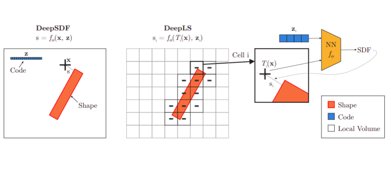DeepLS vs DeepSDF. DeepLS divides the space into a grid and learns local SDF functions.

In order to learn surfaces at scale which would generalize better, DeepLS suggests fusing voxels and DeepSDF. DeepLS grids the space and for each voxel learns a local shape code. All the local voxels share the autodecoder network. Therefore, the network requires to learn a less complex embedding prior and would generalize better to multi object scenes. One caveat of breaking the scene into voxels is how to merge them without getting border effects. DeepLS argues that each code should be able to reconstruct surface from the neighbouring voxels as well, in other words the codes should be locally consistent. Compared to DeepSDF, DeepLS has both impressive quantitative and qualitative results. It is able to reconstruct surfaces that are narrow (higher frequencies) much better. Also, the training time is orders of magnitude faster than DeepSDF.

NGLOD @ CVPR 2021 – arXiv

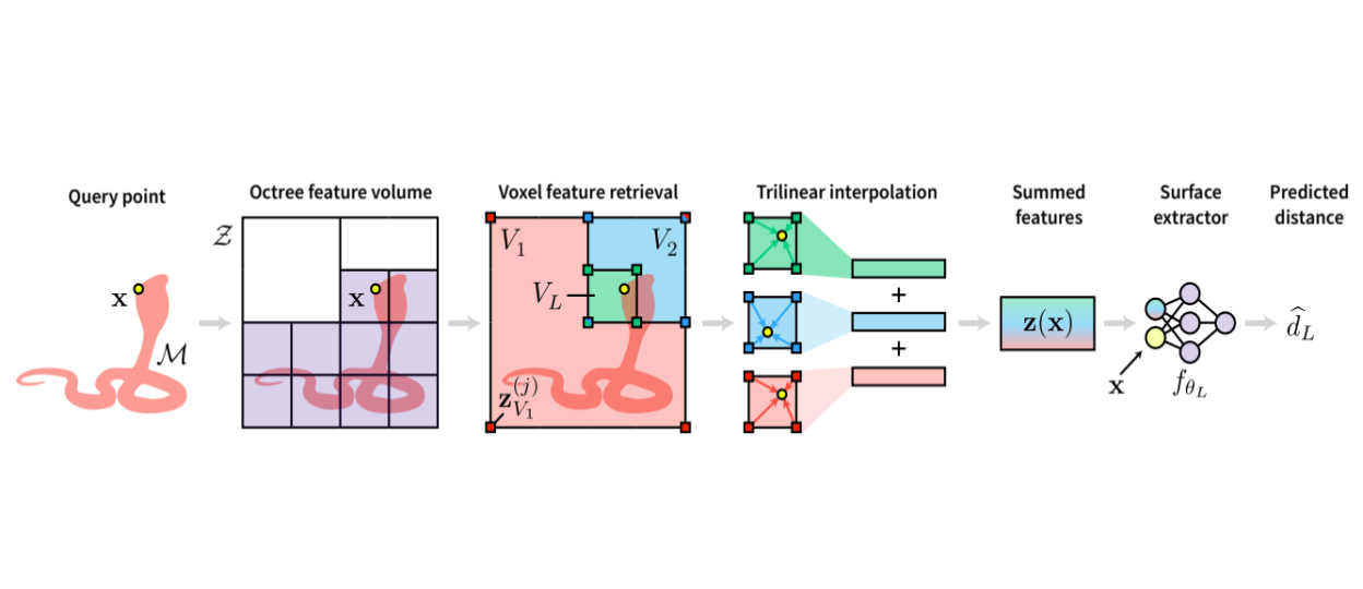NGLOD combines learned embedded values from different LODs using trilinear interpolation at each level.

Neural implicit fields are usually stored in fixed-size neural networks and for rendering there is a computationally heavy and time consuming process of many queries from the network for each pixel. To allow real-time and high-quality rendering, NGLOD uses an Octree based approach to model an SDF function with different levels of detail. At every level of detail (LOD) there exists a grid with certain resolution. For each point the embedded values in the eight corners of all the voxels containing the point, up to the level of detail wanted, are trilinearly interpolated and summed and then passed through an MLP to predict the SDF value. For rendering, because the octree is sparse, a combination of AABB intersection and sphere tracing is introduced. If a point reached by the ray is inside a dense voxel then by sphere tracing using SDF value the surface is found, otherwise the AABB intersection algorithm proceeds to the next voxel. This rendering is super fast and of high quality, but beware! the Octree structure is not learned and consider a priori which means the geometry is not fully learned.

ConvOccNets @ ECCV 2020 – arXiv

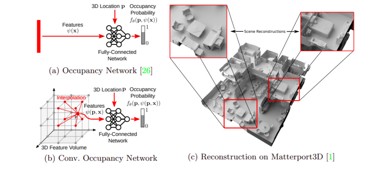*Convolutional Occupancy Networks use CNN to model consistency between embedded features of neighboring nodes. *

ConvOccNet argues that although breaking into local feature grids improves scene complexity and generalization, it would still be beneficial to get context fro the close neighborhood of a node as well. Therefore, ConvOccNets first produce point or voxel features, then they project them into a 2D or 3D grid and process the grid using a UNet. The UNet can propagate information globally over the scene. Then for a specific point features are calculated via bilinear or trilinear interpolation and then passed through an MLP to model the SDF function. Similar to other local works, ConvOccNet is able to learn narrow surfaces or hollow surfaces much better than their global counterpart while also being inherently consistent over grid boundaries. This is due to being able to exploit past experience to inpaint missing parts in the input.

Inverse Rendering Fundamentals

Up to now we discussed 3D neural representations, either overfitting to single scene (NGLOD), or with generalization (OccNet/DeepSDF), but “is it possible to supervise using 2D images only?” This is the objective of inverse rendering. But how can this be achieved? If we assume known geometry, then inverse rendering just needs to memorize view-dependent appearance changes (DNR), while if geometry is not known, we can learn it by either introducing differentiable ray marching (SRN) or differentiable volume rendering (Neural Volumes). As the rendering operation is differentiable, gradients can be back-propagated to the underlying 3D model captured by the 2D images.

Deferred Neural Rendering @ SIGGRAPH 2019 – arXiv

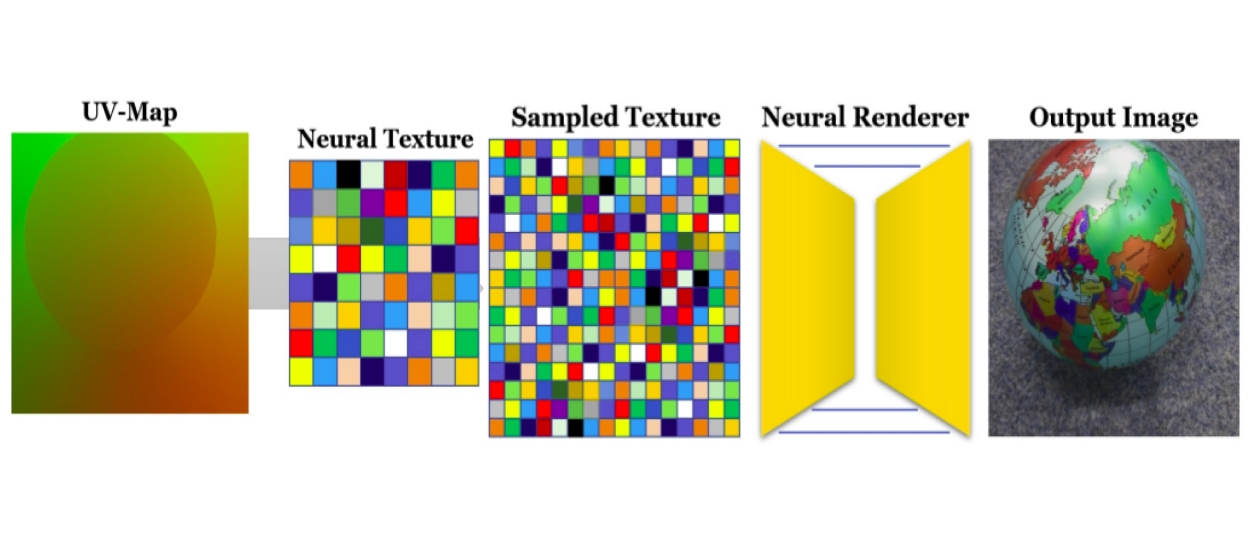:Given an object with a valid uv-map parameterization and an associated Neural Texture map as input, the standard graphics pipeline is used to render a view-dependent screen-space feature map

Detailed and precise texture modeling is essential for a good inverse rendering model. This paper focuses on having learned textures to model view-dependent appearance. The geometry is not modeled and assumed a priori. Unlike traditional texture maps, learned neural textures are used to store high dimensional features rather than RGB that can be converted to pixel color using classic texel-to-pixel pipelines. The texture sampling is hierarchical similar to mimaps to overcome resolution differences. The sampling is made differentiable through bilinear interpolation. One of the distinct and interesting results in this paper is that instead of using a fully connected network as a renderer, using U-Net renderer results in higher quality textures through reasoning about the neighboring areas to have pixel-level consistency.

SRN @ NeurIPS 2019 – arXiv

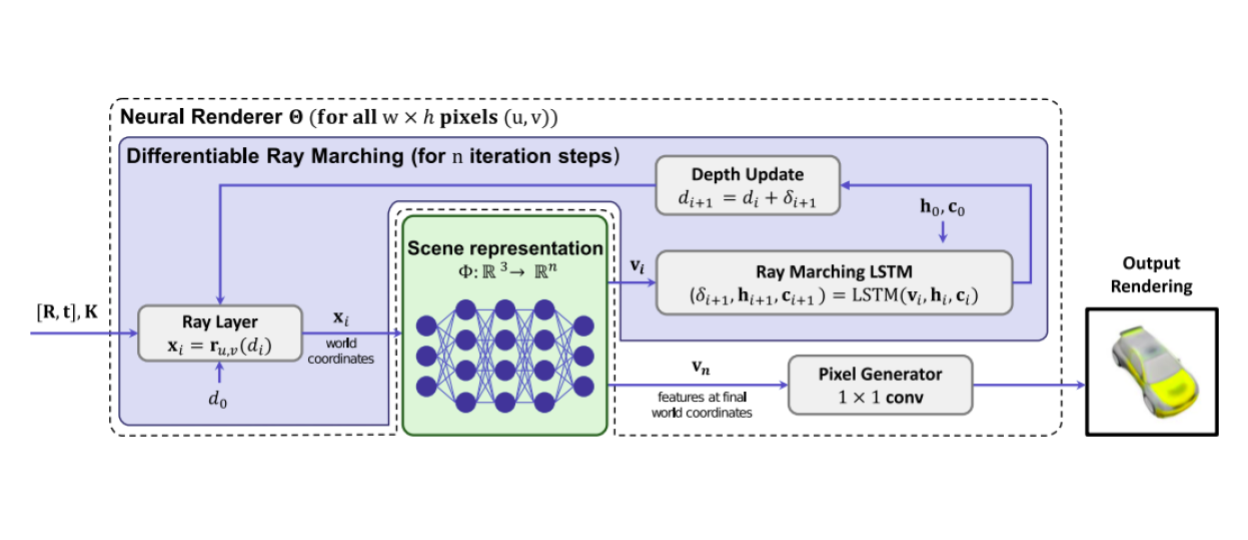SRN achieves inverse rendering of a scene by introducing a differentiable ray marching algorithm based on using LSTM, while memorizing 3D scene eometry and appearance inside an MLP

Joint modeling of shape and appearance in neural implicit fields is a difficult problem. This paper is the first to model 3D coordinate system of a scene from 2D images. The idea is to first identify the surface and then learn the color for the surface. First a differentiable renderer is designed with a differentiable ray marching method that is modeled by a LSTM. The LSTM finds surface depth by iterative refinements. An MLP then maps the 3D coordinate of the point to appearance features and finally RGB color. The colors are not view dependent. This model generalizes to category-level modeling through use of a hyper-net that maps MLP weights to a lower-dimensional sub-space that represents a category’s appearance.

Neural Volumes @ SIGGRAPH 2019 – arXiv

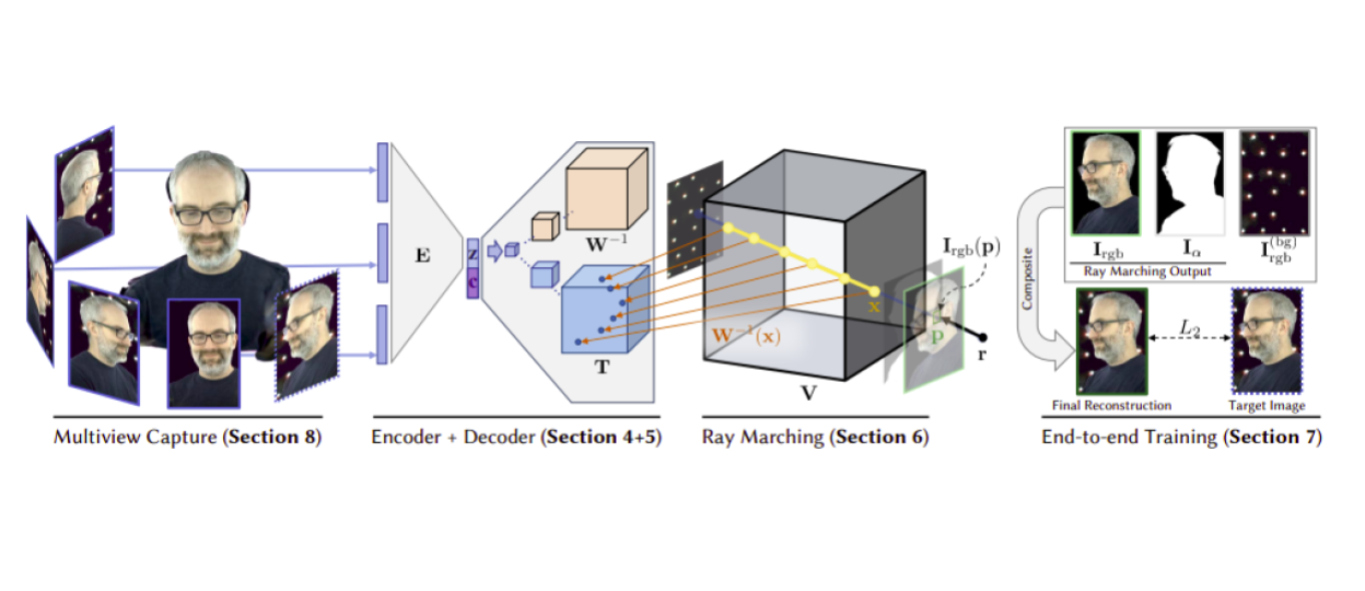Neural Volumes uses volume rendering to achieve novel view synthesis given a set of input images of the scene.

This works aims at rendering new viewpoints from a set of seen viewpoint images. Neural volumes combines volumetric representation learning with ray marching technique to generate realistic and composable renderings. They pass the input images through camera specific CNNs and then combine their latent codes by concatenating and passing them through and MLP. Then decode into a template voxels, a warp field and an opacity 3D grid. They use the warp field to remove the inherent resolution limitation of voxels and be adaptable to different scene complexities at different parts of the space. Finally, they render using accumulating opacity along ray segments in a backpropagateable formulation. This is one of the pioneering works that uses volume rendering to do novel view synthesis. Furthermore, in order to remove smoke-like artifacts they add two regularizers, one on total variation of the opacities and one a beta distribution on opacities. The results are impressively realistic. Since their setup is fixed they also have a background modeling setup. One interesting result they show is that using a learned background image improves the results even compare to giving the ground truth background.

Neural Radiance Fields

A great approach for rendering novel views of a scene or object is to model them as radiance fields which maps each point in space to a view-dependent color and density. These techniques enables learning 3D scenes directly from a set of 2D images.

Volume Rendering Tutorial @ Schloss Dagstuhl 2010 –

This tutorial gives a thorough formulation for different direct volume rendering techniques. Most of the formulations provided in this paper are backpropagateable. Therefore, easily applicable to neural renderings. While Neural Volumes was one of the first papers to use volume rendering, this paper does not assume fixed cameras and formulates volume rendering precisely. The general approach in volume rendering is mapping a 3D scalar field into a 3D field color c and extinction coefficient τ by learning a transfer function (e.g. neural network). Then we can render by integrating along a ray. First, we should define the transparency function T(s) which is the probability that the ray does not hit any particles for a length of s from they ray origin. They drive the formulation for T(s) to be the exponentiated integral of individual extinction coefficients. We can then discretize the formulation by assuming the opacity segments have constant values. This paper refers to several interesting related work that offer more complex formulations without such assumption.

IDR @ NeurIPS 2020 – arXiv

IDR inputs and outputs

Modeling shape and appearance jointly is the goal of many recent papers, with NeRF being the most popular. But this paper achieves this goal by completely disentangling geometry and appearance. This paper models object geometry through first modeling the object’s SDF and then using the inferred surface to pass surface position and normal through a renderer that models object’s appearance. This model is view-dependent and through P-universality: “To model color of a point on object, both view direction and surface normal is needed.” View direction models specularity and surface normal helps to disentangle geometry from appearance and be able to model deformations in the object too! With this formulation a renderer learned on an object can be attached to SDF of another object to give the appearance and material’s look of one object to another. The paper further can refine the camera parameters by back propagating all the way back to view direction and point position and shows promising results for pose estimation.

NeRF @ ECCV 2020 – arXiv

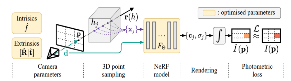
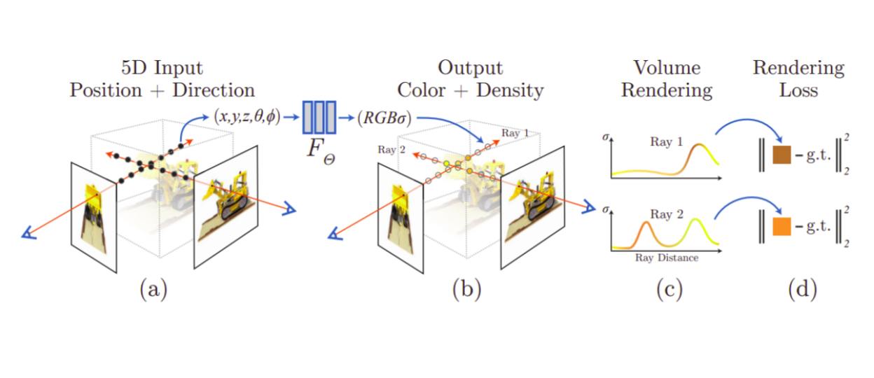NeRF process: samples points along the rays, queries RGB and opacity, and finally composites them by integrating along the ray i.e. volume rendering.

This work is the culmination of techniques we have discussed thus far. The goal is similar to Neural Volumes, rendering new viewpoints from a set of seen images. They employ volume rendering techniques and use an MLP as the transfer function to map 3D points in space to view-dependent color and density. Nerf also has hierarchical aspects as in it trains on both coarse and fine scale. Nerf does not face boundary issues like what was discussed in DeepLS since they sample points randomly rather than having a set of fixed positions. A simple MLP however would still suffer from the oversmoothness because of its spectral bias. Nerf alleviates this shortcoming by augmenting the 3D point coordinates with positional encoding at different sinusoidal frequencies. The positional encoding again shows the importance of explicit multiplicative conversions done before passing input to MLP, which is the main idea and reason of success in transformers, too. Also, similar to Neural Volumes, Nerf conditions the rgb generation on the view direction to better handle viewpoint dependent artificats. Combination of all these techniques results in far superior renderings in a much less restricted setup compared to prior works such as Neural Volumes. Despite major success, this work has limitations like requiring too many input views, perfect camera calibration, static objects and modeling just a single scene.

Neural Light Fields

Although radiance fields are great at modeling appearance they fail in certain cases. For surface rendering, in the case of a non-solid object the modeling fails and for volume rendering, when the viewing ray does not necessarily travel along a straight line (e.g. refraction) the model fails. 4D light fields are the models that are capable of modeling these failure cases but only when applied scenes viewed from outside their convex hull. In 4D light fields for every viewing direction only one value of radiance is stored and hence the model only memorizes a mapping from view direction to radiance (i.e. the output of integration in NeRF volume rendering), not caring for solidness of surfaces, volumetric properties or accumulated color like surface/volume rendering. For this same reason it is incapable of modeling occlusion, it is not 3D consistent and fails to capture occluded surfaces. In LFN and LFNR we see different parameterization of light fields and how well they work on specularity and refraction in both forward-facing and 360 degree scenes. Learning Neural Light Fields, we see an important idea on combining light fields with explicit grids and how to some extent that helps overcome occlusion problem in light fields.

LFN: Light Field Networks @ NeurIPS 2021 – arXiv

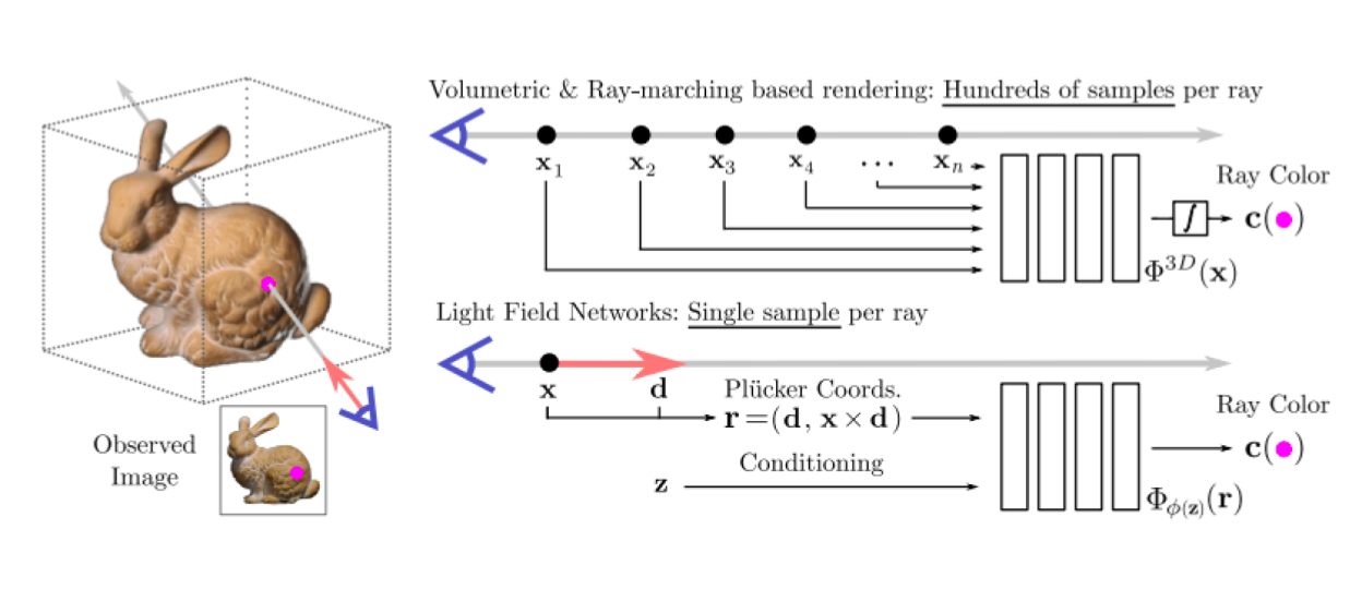Getting pixel color from LFN through only one network query

The classic parametrization of light fields limits these fields to forward facing or other constrained spaces and does not allow for 360 degrees modeling of the scenes. In this paper a new parameterization for 4D light fields is introduced. This parameterization is based on the 6-dimensional Plücker coordinates in which light fields lie on a 4-dimensional manifold. This parametrization allows or 360 views of scenes unlike the traditional parametrization of light fields. The 6D coordinate is taken as input to a MLP and ray color is given as output. Again, because there is no volume rendering or integration, a pixel color can be found through only one quey of the network. At last a meta-learning approach based on hyper-network training is proposed to generalize to different scenes.Simple 3D senes can be modeled when a single shot is given as input. For this task the comparison to SRN is interesting, where modeling sudden discontinuities (like holes) is hard for SRN, this model overcomes that problem.

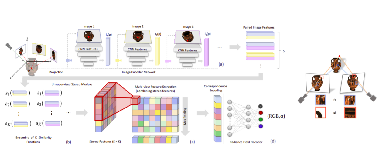
Light Field Neural Rendering @ CVPR 2022 – arXiv

LFNR uses two transformers to model light fields, one extracts features from points along a given ray and another reasons between corresponding points projected to different reference views.

This work models 4D light field with the use of transformers. Given a sparsely observed scene, this method uses epipolar geometry constraints (much like IBR) to model geometry with help of a transformer and then view-dependent appearance of a light field through a second transformer. Two closest reference views to target view are selected and the sampled points along target rays are projected onto them. The first transformer decides which one of the sampled points on the ray is closest to the query point by predicting attentions. The second transformer decides which of the reference view directions to pay more attention to. This work is an interesting use of transformers in neural implicit fields and the results show impressive modeling of reflection and refraction. Because there is no volume rendering and integration, here the network is able to model inconsistencies like refraction between different views and memorize them. Compared to the previous paper this model gives crisper results but takes a long time to train due to use of transformers.

Learning Neural Light Fields @ CVPR 2022 – arXiv

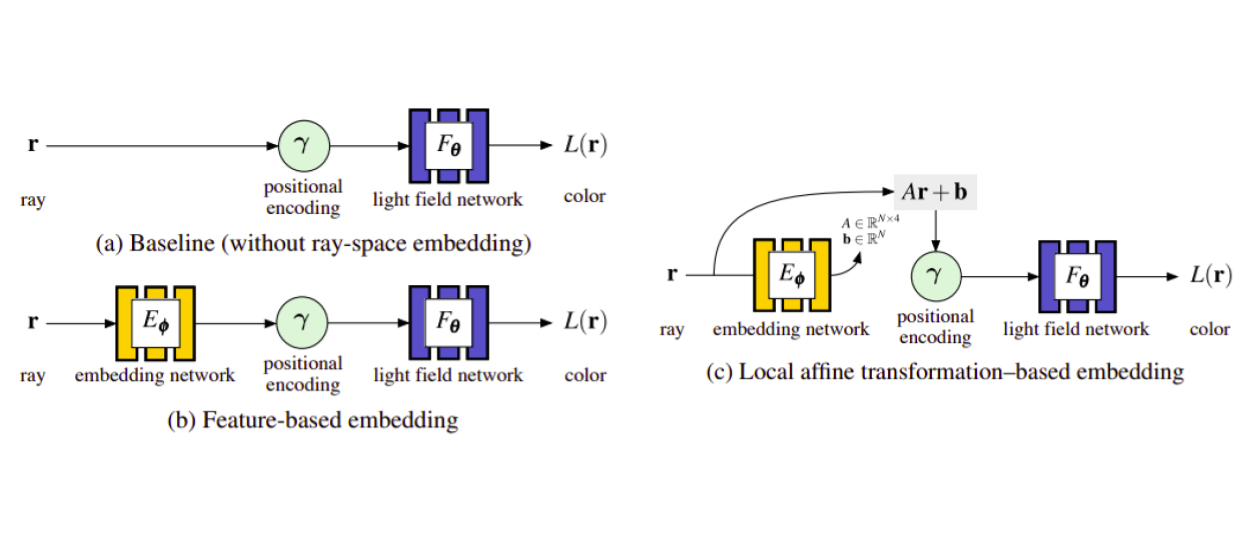Local Light Fields uses grid embeddings to align ray planes using affine transform.

By now we know that 4D light fields are inherently not consistent in 3D and the associated color value for each ray is memorized independently of other rays. This paper’s solution for this problem is first to add an embedding network before the positional encoding to align and affine transform the ray planes. They subdivide the space into local voxels and learn local light fields and render based on the opacity of ray portion when it hits a voxel. Given the constant radiancy and forward facing assumptions this method results in better modeling of shiny or reflective surfaces compared to Nerf, while handling occlusions and views from outside the convex hull of the scene to some extent.

Image Based Rendering

The methods in this section are designed to condition volume rendering on few images. The design decisions are mainly around how to formulate the conditioning while keeping the model fast to infer. When given a new scene, there is no need for training and a novel view can be queried from reference views by projecting query points onto them and feature matching.

pixelNeRF @ CVPR 2021 – arXiv

PixelNerf conditions on input images to generate 3D point feature vectors.

In order to achieve generalizability over scenes NeRF input needs to be conditioned. PixelNerf conditions NeRF on a few images by finding the corresponding feature vector of the sampled point from a closed-form projection of the input image. So in addition to position and viewpoint, PixelNerf concatenates a bilinearly intorpolated feature vector extracted from the input images. In case of conditioning on multiple input images, each feature vector is processed first with a shared MLP and then average pulled and processed with one more MLP block. The average pulling gives this pipeline permutation covariance. The results show that for the cases with less than 6 images, pixelNerf provides a significant gain.

Stereo Radiance Fields @ CVPR 2021 – arXiv

Left: Stereo Radiance Field pipeline, Right: Intution for inferring radiance out of stereo image projection

In this paper, given a set o sparse stereo reference images of a scene, density and radiance of each point is predicted by finding correspondence to that point in the reference images. A comparison based learnable module is introduced that given a point on the novel view, compares the features extracted from the projected point on to reference views. If the features align then the point is on an opaque unoccluded surface hence has high density value and similar RGB value, otherwise it is probably in the air and has small density. A learnable module compares feature vectors across all reference views and find correspondences (stored in a vector) which is then passed to an MLP to output RGB and density. After that the NeRF volume rendering is performed. The comparison module learns useful comparison metrics to find correspondences and can be transferred to unseen scenes for generalization. To further increase quality, it can be fine-tuned on that scene. A failure case is when trying to model reflections and texture-less regions where finding correspondence is naturally hard.

SRT @ CVPR 2022 – arXiv

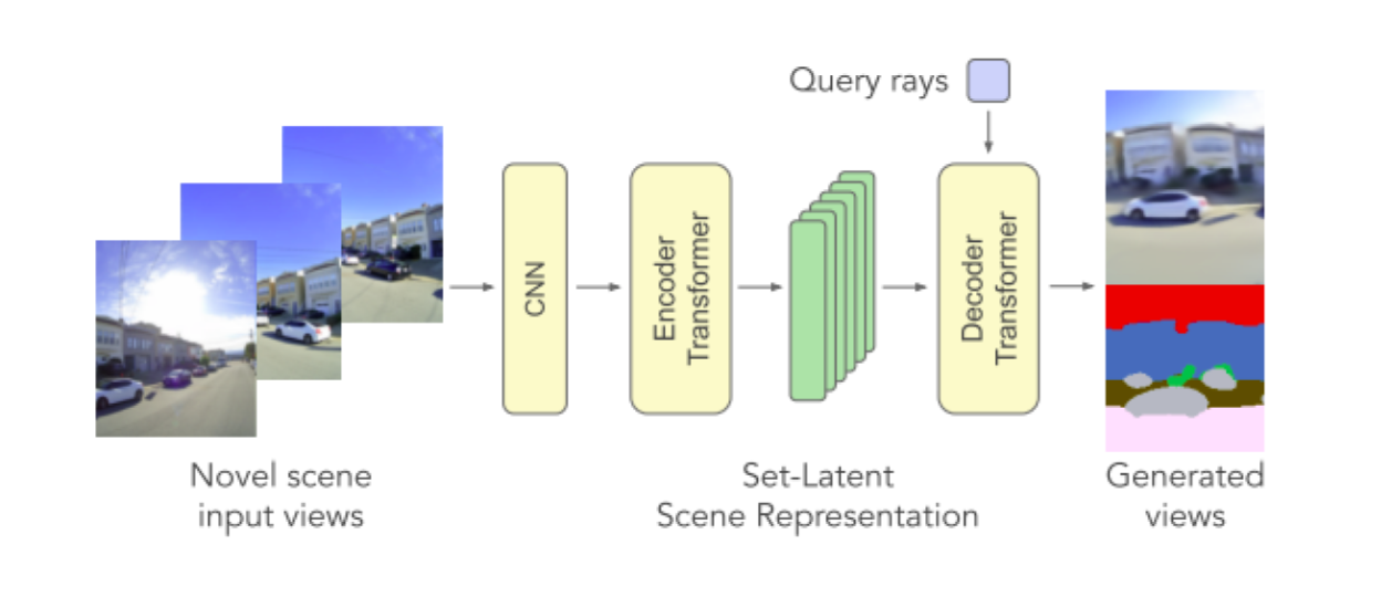SRT procedure: ViT encoder + Transformer decoder.

SRT uses a ViT as the encoder by patching and running attention-transformer blocks. This enables better aggregation over input images as opposed to average pooling in PixelNerf. But SRT relies on patches as in ViT rather than exploiting direct point features of PixelNerf. Another important aspect is rather than typical Nerf models, which concatenate viewpoint to the position for decoding, SRT uses attention with the ray viewpoint as the query and introduces a new architecture for neural fields. As a result of this changes they are able to outperform prior work like PixelNeRF or LFN, especially when seen viewpoints are not hand selected and the novel viewpoint is farther away from the seen viewpoints.

Multi Resolution

Vanilla NeRF is only capable of modeling scenes at a certain resolution and in a bounded domain. What happens if we want to model scenes in different resolution when viewing camera is not set at only one certain distance from center of the scene? For real scenes NeRF only handles the forward facing views with unbounded range, but is it possible to model high-quality unbounded scenes with 360 degree views? Here we see how the aliasing problem is handled when multi-resolution images are inputs to NeRF (mip-NeRF), or how to handle this problem with the use of a multi-resolution grid (NSVF). Mip-NeRF-360 proposes solutions for modeling unbounded scenes while not losing high-quality rendering in NeRF.

NSVF @ NeurIPS 2020 – arXiv

Self-Pruning for different LODs during training

This paper, very much like NGLOD, but in the realm of NeRFs. Here they explore the idea of hierarchical NeRFs to speed up rendering. Using just one MLP and doing volume rendering through hundreds of queries for each ray is slow and computationally expensive. Space is modeled as an explicit voxel grid and there exists tiny MLPs for each voxel that process the embedded values at the 8 corners. Through the learning process voxels with lower densities are pruned and the radiance is therefore stored in an octree of embeddings passed through a tiny MLPs (here the structure of octree is actually learned through pruning unlike NGLOD). Therefore the rendering is very fast and is done through an AABB intersection process to find the voxel containing the surface hit by a ray and then the color of the surface is extracted from that voxel by a forward pass of a small MLP. The quality of reconstruction is impressive and can beat baselines like NeRF and SRN with higher levels of LOD while having faster renderings. Some limitations are being prone to over-pruning and not modeling complex backgrounds.

Mip-NeRF @ ICCV 2021 – arXiv

NeRF ray tracing vs MipNeRF cone tracing

Volume rendering in NeRF requires sampling points along a viewing ray. The typical approach is to have a two phase course and fine sampling strategies and relearn the implicit function to avoid aliasing. MipNeRF suggests rather than a narrow ray, we consider a cone with a base of pixel width. Then we can integrate the points in frustums to get an approximate color/density. They approximate the frustum with a multivariate Gaussian and then transform them into the expected positional encoding of the points in the frustum. This method encodes the scale of frustums in the positional encoding which results in better disambiguation and antialiasing. Also, since they train a single network rather than a course and a fine version they are potentially faster.

Mip-NeRF-360 @ CVPR 2022 – arXiv

Left: Hierarchical importance sampling scheme, Right: Coordinate reparameterization into a bounded radius

NeRFs fail in modeling unbounded scenes for multiple reasons, the most important being the linear parametrization of space that leads to infinite depth for unbounded scenes and also the not robust importance sampling scheme that does not scale to bigger scenes. Although NeRF models real unbounded scenes of LLFF dataset, it does so only for forward-facing scees that can be parametrized in a bounded way using NDC conversion. The contributions of Mip-NeRF-360 is three-fold. First, a new parameterization for the space is introduced to model unbounded scenes. The foreground is parametrized linearly as before, but the background is contracted (based on inverse depth) into a bounded sphere of fixed radius. Therefore distant points are distributed proportional to inverse depth i.e. the further the less detailed the scene becomes. A compatible sampling method is introduced to sample uniformly in inverse depth. Second, a hierarchical scheme is used for importance sampling. Two MLPs are used, one proposal MLP used for sampling and the other NeRF MLP used for rendering. The NeRF MLP works as before, but the proposal MLP tries to estimate weights that show the distribution of important segments sampled along the ray. This distribution is then sampled and points are passed to NeRF MLP for rendering. The proposal weights are supervised through a propagation loss that penalizes proposal weights that underestimate NeRF weights. This loss only affects the proposal MLP and the gradient back-prop is not applied to NeRF MLP. Lastly, a new regularizer for suppressing floaters is introduced that encourages mass being centered closely mostly at one point over the ray.

Fast Training

Having a set of fixed evaluation points as in voxel training enables much more efficient GPU utilization and leads to faster training times. Radiance Fields though rely on evaluating several random points along the ray. A compromise is proposed in this section’s set of works by interpolating trainable embeddings. The general consensus is that having a non-linearity after the interpolation is a must for getting high-quality results.

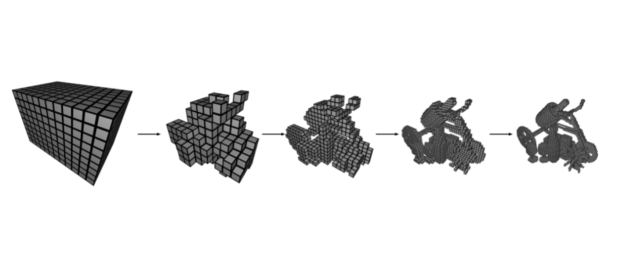
InstantNGP @ SIGGRAPH 2022 – arXiv

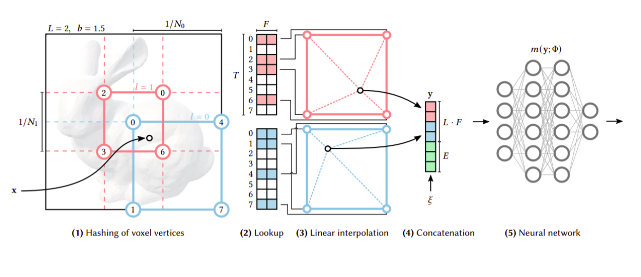InstantNGP speeds up training by hashing the voxel corners and interpolating their learned embeddings.

In order to improve the training speed and memory consumption without relying on tree structures, instant NGP proposes having a hierarchy of fixed voxel grid positions. A certain 3D point is then embedded as the interpolation of the features of the voxel corners around it. The embeddings from different levels are then concatenated and passed through an MLP similar to regular NeRF training. Since each point has several levels and corners the MLP can implicitly resolve any hash collisions. Using trainable embeddings allows for a very shallow and narrow MLP (2 layers of 64 neurons). Also hashing, looking up at fixed points, and interpolation enables fascinatingly optimized implementation over GPU.The result is very sharp and high quality results in less than a minute of training, which essentially makes it a real time renderer. Furthermore, they keep an occupancy grid to guide their sampling strategy and avoid wasted computation as opposed to MipNeRF which uses an MLP to model occupancy.

Plenoxels @ CVPR 2022 – arXiv

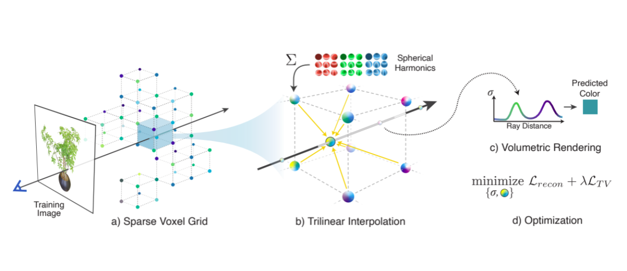Plenoxels speedup the training by replacing the MLP with interpolating corner embeddingss in a sparse voxel grid.

In Plenoxels this problem is addressed by completely getting rid of the neural nets and instead using an explicit grid with embedded values for density and spherical harmonics (basis to encode RGB value) in the eight corners of each cell. This paper also uses ReLU on the embedding values and then passes it to a bilinear interpolation similar to ReLU Fields. The predicted density and RGB is then passed through volume rendering. Because of querying regular grids this is much faster than network based volume rendering although it still used hundreds of queries for each pixel. The grid is pruned for faster and lower number of queries. Additionally different regularizers are introduced that prove useful for learning correct and robust geometry.

ReLUFields @ SIGGRAPH 2022 – arXiv

Representing a ground-truth function (blue) in a 1D (a) and 2D (b) grid cell using a linear function (yellow) and a ReLUField (pink). ReLUField can capture the discontinuity more accurately.

Having a set of regular grid positions, learn embedding for those fixed points, and then interpolate them is much faster than running an MLP on a huge set of randomly sampled points along all the rays. But the MLP adds flexibility to the modeling both in terms of high frequency modeling and view dependent effects. ReLUFields suggests by just adding a ReLU non linearity after the interpolation. They also incorporate the coarse to fine training regime by first training at low resolution grid size. Then they upsample using trilinear interpolation and continue training. They use the same formulation as NeRF. By using a regular grid based representation rather than an MLP, at about 10 minutes of training time ReLUFields are able to match the results of original Nerf which is trained for several hours.

Camera Extrinsics

With NeRF training becoming increasingly fast, the bottleneck of NeRF training is running unposed images through COLMAP to get camera parameters. The line of work in this section explores ideas and challenges of jointly optimizing camera parameters along NeRF and show promising results.

BARF @ ICCV 2021 – arXiv

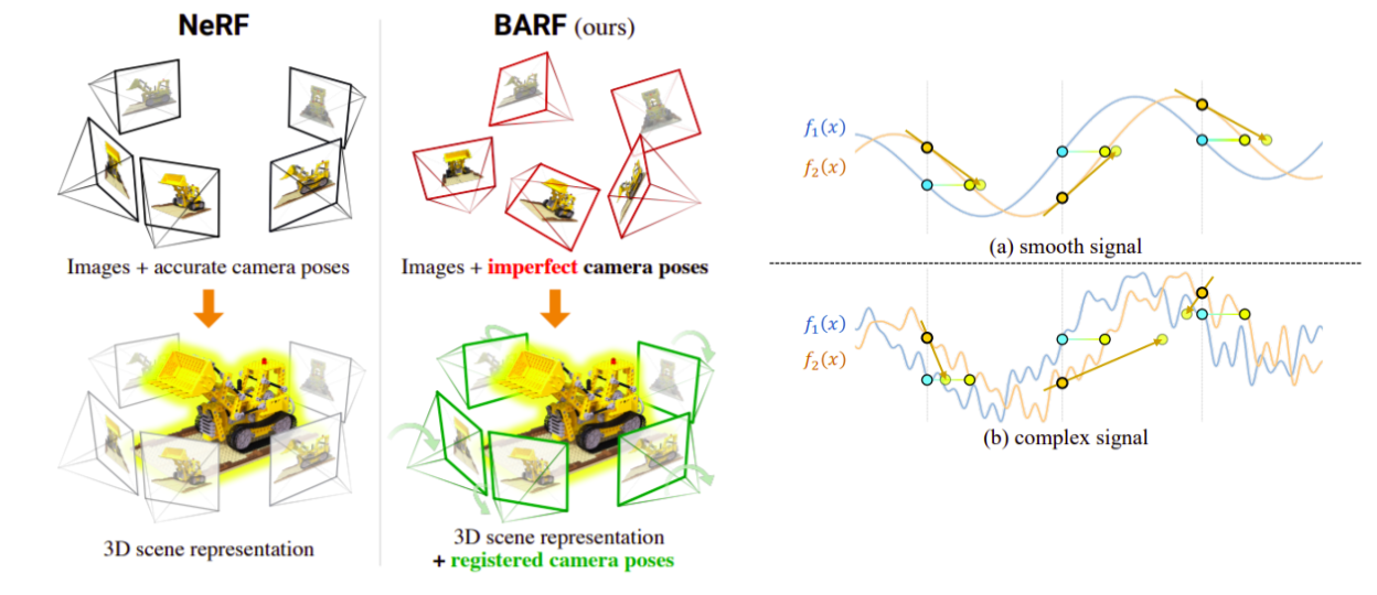Left: BARF is robust to imperfect camera poses and is able to jointly register the camera poses and train the NeRF model. Right: Signal displacement prediction is much easier in smooth signals hence BARF uses a course-to-fine alignment process.

Casting rays (mapping 3D points to pixeles) requires camera calibration. What can we do if we don’t have the calibration parameters? The good news is that the transformation from camera parameters to 3D points is potentially backpropagatable. The bad news is that due to the positional encoding, different frequencies receive disproportionate gradients. Therefore, BaRF suggests having different learning curriculums for different frequencies. They add a weight factor to reduce the gradient from the high frequencies at the start of training. The results on real scenes suggest that it can match the performance of SFM methods and render well aligned images with their bundle adjustment technique. The caveat is having to deal with extra hyper parameters for scheduling the optimization is tricky.

Nerf- - @ Arxiv 2021 – arXiv

Nerf-- : Camera parameters are learned alongside network weights

To grasp the difficulty level of learning a NeRF with unknown camera parameters, this paper analyzes learning camera poses and intrinsic parameters jointly with NeRF weights. All of the experiments are done on forward-facing scenes to simplify the problem and yet it is shown that in many cases if the camera path is slightly perturbed the camera pose estimation fails (and sometimes COLMAP also fails in this scenario!). This paper along with providing a dataset with perturbed camera poses, shows that joint learning of camera parameters and NeRF weights is trickier than just setting these parameters as learnable variables.

GARF @ Arxiv 2022 – arXiv

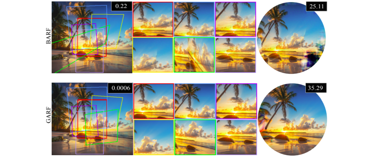Comparison of BARF and GARF

Due to spectral bias of MLPs, learning high frequency data on vanilla MLPs is hard. To solve this NeRF uses positional encoding that maps positions to higher frequency spectra and forces MLP to learn detailed high frequency data. One disadvantage of this approach is that the high coefficients used in positional encoding, dampens the gradients in the backpropagation, if camera parameters are needed to be optimized. Although BARF, shows a coarse-to-fine learning method that gradually adds on the higher frequencies, this method needs careful scheduling. In GARF, the positional encoding is removed and Gaussian activation is used instead of ReLU in the MLP.

It is mathematically shown that this Gaussian-MLP is able to learn high frequency data and has a nice back-prop process that helps with camera pose estimation.

Learnable Appearance

NeRF excels in controlled and static scenes. In practice such meticulously gathered datasets are not always available. For example given a set of photos of a tourist attraction site such as Eiffel tower (i.e. photo tourism datasets), the ambient light and transient objects such as pedestrians invalidate the NeRF assumption of a static scene. The papers in this section utilize robust losses, bundle adjustment techniques, and trainable embedding vectors to model such variations in the dataset.

NeRF in-the-wild @ CVPR 2021 – arXiv

Nerf in the wild uses an appearance embedding to allow for per image change and a transient MLP tower to model redundant objects.

Nerf models fail in an uncontrolled setup such as a collection of images on the internet. The main reason is Nerf assumes the color intensity of a point is the same from different viewpoints. But in a random collection of images of a scene there are both photometric variations such as illumination and transient objects (e.g. moving pedestrians). These techniques enables Nerf-w to handle appearance change and transient objects while still generating sharp objects. Nerf-w tackles the photometric inconsistencies by learning a per-image embedding and concatenating it to the input of the MLP. Essentially making the color prediction not only view dependent but image dependant as well. To handle transient objects, Nerf-w has another MLP which outputs another set of color and occupancy alongside uncertainty modeled by normal distribution. They estimate the variance of the normal distribution to be both image and view dependant. Therefore, they learn another set of image based embedding vectors. Nerf-w simply adds an L1 regularizer to the transient density to avoid explaining away of static scene with transient parts.

Nerfies @ ICCV 2021 – arXiv

Nerfies uses a deformation field to map into the canonical coordinate of the object and allows for per image appearance change.

Given that Nerf only works in static and controlled setup, what happens if the object of interest is deformable? Nerf fails since the color to 3D point assignment varies between images. Nerfies models the deformability of an object explicity by learning a warp field. A per image embedding is used to SE(3) transform points from that image coordinate frame into the canonical coordinate frame. The warping field introduces many ambiguities in the optimization. Nerfies incorporates and elasticity regularizer which forces the singular values of the Jacobian of the deformation to be close to identity. Also, SE(3) assumes rigidity which does not hold in all situations therefore rather than L2 optimization, they use a Geman-McLure robust loss function on the singular values of the Jacobian. Also assuming access to a set of fixed background points they add background regularization. They also incorporate bundle adjustment techniques and clamp the trainable frequencies with a schedule during training similar to BaRF. The results show that BG modelling and SE(3) enforcement are the most impactful adjustments while all the design decisions having impact in some situations.

HyperNeRF @ SIGGRAPH Asia 2021 – arXiv

HyperNerf slices a hyperspace using deformation and ambient fields rather than a 3D space. Also, using an appearance embedding Hypernerf accommodates per image appearance change.

If the object of interest moves, nerf fails to align the rays, points, and pixels and the optimization fails. In this work they tackle the challenge of non-rigid topologically changing objects. HyperNerf models a hyperspace of the 3D volume. Each image has an associated trainable warping embedding. They model a deformation field with an MLP and the ambient changes with another MLP. Therefore mapping the original 3D point into a canonical hyperspace. The deformed point and the ambient slice are positionally encoded and passed through the NeRF MLP and optimized with volume rendering. At inference they can both change appearance by moving in the topography plane and in the spatial plane.